Implementing Stochastic Gradient Descent in C++ for Supervised Learning on Data with Sparse Features
This post cannot be read on its own. One need to read the previous blogpost about implementing Gradient Descent where we learn how to implement Gradient Descent to solve a supervised (binary classification) learning problem. The coding up of the loss function has been explained in good detail there. The post also talks about how to read the sparse classification datasets into compressed row storage sparse matrices and how to use these data structures to solve the supervised learning problem using Gradient Descent. I assume you have taken a look at the previous post and I will jump right into implementing the stochastic gradient solver part.
Let us try to use the following steps of Stochastic Gradient Descent at an epoch $t$ (as usual we choose the first guess as an all zero vector).
Step 0: Given $x^{t}$
Step 1: for iter = 1, … , m, do the following: (Remember, there are m samples):
Step 1a: choose $i \in {1, \dots m} $ randomly
Step 1b: compute the gradient of $L$ at the current observation and current $x$. i.e. $g = L’(x^{t}:a_{i},y_{i})$
Step 1c: We update the learning rate as follows $\eta = \frac{1}{1+t}$
Step 1d: update $x \gets x −\eta (g+\lambda x)$
Step 2: $x^{t+1} \gets x$
The above pseudocode is taken (and slightly modified) from lectures notes of Martin Takac.
The SGDSolver.hpp file looks like this
#ifndef SGDSolver_hpp
#define SGDSolver_hpp

#include <stdio.h>
#include "CoreSolver.hpp"

#include <random>
#include <chrono>

class SGDSolver : public CoreSolver{

public:
    std::vector<double> x;
    std::vector<double> grad;
    std::vector<double> ATx;
    double lambda;
    double eta;
    int epochs;

    //Just some variable for random integer generation.
private:
     std::random_device rd;
     std::mt19937 rand_gen;
     std::uniform_int_distribution<int> distribution;
public:
    virtual void init(const Classification_Data_CRS &A, double lam, double alfa, int max_iter);
    virtual void run_solver(const Classification_Data_CRS& A);
    virtual void run_one_stochastic_epoch(const Classification_Data_CRS &A, std::vector<double>& x, int iter_counter);
    virtual void run_one_iter(const Classification_Data_CRS &A, std::vector<double>& x, std::vector<double>& ATx, std::vector<double>& grad);
};


#endif /* SGDSolver_hpp */
We can see that SGDSolver is a child class of CoreSolver. The biggest difference is the random number generator and we have a new function which runs a stochastic epoch.
We use standard C++11 way to generate the random numbers and let us see the implementation of the header function files.
void SGDSolver::init(const Classification_Data_CRS &A, double lam, double alfa, int max_iter){

    (void) alfa;
    (void) lam;

    x.resize(A.n, 0); //We are creating a vector of all 0s of size n (number of features)
    grad.resize(A.n, 0); //The gradient also is of size n
    ATx.resize(A.m, 0); //This vector holds the value of A*x. (T is times and not transpose)
    lambda = 1.0/A.n;
    eta = 1.0;
    epochs = max_iter;

    auto seed = rd();
    rand_gen = std::mt19937(seed);
    distribution = std::uniform_int_distribution<int>(0, A.m-1);

}
The above function is just an initialization function. We set the values of lambda and eta (I think I used alpha for gradient descent ) differently here. So we do not use the given by the user (we can change this behavior, at least for lambda as eta is always 1 when starting). Then we create the random number generator, distribution. We create 0 vectors of respective sizes for x, grad and, ATx.
The next function is to run the solver
   1  void SGDSolver::run_solver(const Classification_Data_CRS &A){
   2
   3     // At the begenning, we just have the x varibale which will be updated in each epoch and within each epoch,
   4     // the x variable should technically be updated at each sample that has been analysed.
   5
   6     //Let us first set up the variables
   7     LogLoss::compute_data_times_vector(A, x, ATx);
   8     double obj_val =  LogLoss::compute_obj_val(ATx, A, x, lambda);
   9
  10     double train_error = LogLoss::compute_training_error(A, ATx);
  11     LogLoss::compute_grad_at_x(ATx, A,x, lambda, grad);
  12
  13     //Setting up the output that would be visible on screen"
  14     std::cout << "   Iter  " <<  "    obj. val  " << "     training error "  << "        Gradient Norm  " << "\n";
  15     std::cout << std::setw(10) << std::left << 0 << std::setw(20) << std::left << std::setprecision(10) << obj_val << std::setw(20) << std::left << train_error << std::setw(20) << std::left << get_vector_norm(grad)<< "\n";
  16
  17
  18     //Now let us run the solver for all the epochs
  19     for(int t = 1; t <= this->epochs; t++){
  20
  21         this->run_one_stochastic_epoch(A, x, t);
  22         LogLoss::compute_data_times_vector(A, x, ATx);
  23         obj_val =  LogLoss::compute_obj_val(ATx, A, x, lambda);
  24         train_error = LogLoss::compute_training_error(A, ATx);
  25         LogLoss::compute_grad_at_x(ATx, A,x, lambda, grad);
  26         std::cout << std::setw(10) << std::left << t << std::setw(20) << std::left << std::setprecision(10) << obj_val << std::setw(20) << std::left << train_error << std::setw(20) << std::left << get_vector_norm(grad)<< "\n";
  27
  28     }
  29
  30 }
Lines 7-12 are just setting up for the first line of logging and lines 13-14 set up log the first iteration. Line 19 runs the algorithm for the user-supplied number of epochs. We then run a single stochastic epoch and we get a new value of $x$. Then we log the updated objective function value and the training error. And we do this for the given number of epoch and hope that we have a good solution.
So.. Probably the most important function is running a single statistic epoch.
   1 void SGDSolver::run_one_stochastic_epoch(const Classification_Data_CRS &A, std::vector<double> &x, int epoch_counter){
   2
   3     //    The pseudocode for running one epoch is:
   4     //    input x_t  (at t epoch)
   5     //    set x <- x_t
   6     //    for it = 1, ... , m do:  //There are m samples
   7     //        choose i in (1,..,m) randomly
   8     //        compute the gradient at the single ( y_i, a_i ) observation               //  Step 0
   9     //        set η = 1/(1 + t) // t^th epoch and m samples and i^th sample             //  Step 1
  10     //        update x = x - η(g + λx)                                                  //  Step 2
  11     //    x_t+1 <- x_t
  12
  13
  14     //    It is important to realzie that step 2 changes all the coordinates of x and for very sparse x,
  15     //    the gradient is gonna be sparse and we have to do a sparse update.
  16
  17     auto scale = 1.0;
  18
  19     for ( auto it = 0; it < A.m; it++){  //iterating through the m samples
  20         //Let us get a random integer between 0 and m
  21         auto random_obs_index = distribution(rand_gen) ; //Store the observation number which is going to be used.
  22
  23         //Step 0. The stochastic gradient is going to be be computed here itself.
  24         //The  gradient  L'(x; a_i, y_i) at (a_i, y_i) looks like this
  25         //
  26
  27
  28         //                                                 [  ai_1*y   ]
  29         //                                                 [  ai_2*y   ]
  30         //                                 (-y*aTx)        [  ai_3*y   ]
  31         //                                e                [    .      ]
  32         //         L'(x; a_i,y_i) = ------------------     [    .      ]
  33         //                                    (-y*aTx)     [    .      ]
  34         //                               1 + e             [    .      ]
  35         //                                                 [    .      ]
  36         //                                                 [  ai_n*y   ]
  37         //
  38         //                          :__________________:  :______________:
  39         //                              factor_1             sparse a_i
  40         //
  41
  42         //        To compute this gradient, the quickest way I can think of now is to loop though sparse a_i twice
  43
  44
  45         auto y = A.y_label[random_obs_index];  //Stores the y value of that random_observation chosen
  46         // To calculate the  factor_1
  47         auto rand_aTx = 0.0;
  48         auto factor_1 = 0.0;
  49         for(auto i = A.row_ptr[random_obs_index]; i < A.row_ptr[random_obs_index+1]; i++){
  50             rand_aTx += A.values[i]*x[A.col_index[i]];
  51         }
  52         factor_1 = (-1.0*y)/(1.0+exp(y*rand_aTx));
  53
  54 //        grad.resize(A.n, 0);  //Most likely not needed
  55
  56         for (auto i = A.row_ptr[random_obs_index]; i < A.row_ptr[random_obs_index+1]; i++){
  57             grad[A.col_index[i]] = factor_1*A.values[i];
  58         }
  59         // We have the gradient values in the respective coordinates. now let's calculate the eta.
  60         eta = 1.0/(1.0+epoch_counter);
  61
  62         // The update x = x - η(g + λx)   is slightly tricky. We can write it as follows:
  63         // x = x -ηλx -ηg => x = (1 -ηλ)x -ηg. On face of it, it is changing every single coordinate of x and can not do a sparse update. But we can use
  64         // a scaling trick to make a sparse update.  The following matlab code gives an idea how to do it. We choose a scale 's' and rescale g (gadient) using 's' and update the
  65         // scale at every iteration. Then we will multiply the final w with the updated scale.
  66
  67         //                    Changing all coordinates
  68         //                    w = [0 0 0 0 0]';
  69         //                    g1 = [0 1 0 1 0]';
  70         //                    g2 = [0 0 1 0 1]';
  71         //                    g3 = [1 0 1 0 0]';
  72         //                    lam = 2;
  73         //                    n1 = 0.2;  n1 is the eta in first iteration
  74         //                    n2 = 0.3;  n2 is the eta in second iteration etc.
  75         //                    n3 = 0.4;
  76         //
  77         //                    w = w-n1*(g1+lam*w);  // updating all the coordinates 1st iter
  78         //                    w = w-n2*(g2+lam*w);  // updating all the coordinates 2nd iter
  79         //                    w = w-n3*(g3+lam*w);  // updating all the coordinares 3rd iter
  80         //                    w_all = w;
  81         //
  82         //                    sparse update with scaling
  83         //                    w = [0 0 0 0 0]';
  84         //                    s = 1;   %scale
  85         //
  86         //                    s = s*(1-n1*lam);
  87         //                    w(2) = w(2) - (n1/s)*g1(2);    //We know that only 2 and 4 cooridnates are non-zero in gradient/
  88         //                    w(4) = w(4) - (n1/s)*g1(4);
  89         //
  90         //                    s = s*(1-n2*lam);
  91         //                    w(3) = w(3) - (n2/s)*g2(3);
  92         //                    w(5) = w(5) - (n2/s)*g2(5);
  93         //
  94         //                    s = s*(1-n3*lam);
  95         //                    w(1) = w(1) - (n3/s)*g3(1);
  96         //                    w(3) = w(3) - (n3/s)*g3(3);
  97         //
  98         //                    s*w
  99         //                    w_cor
 100
 101         scale = scale*(1-lambda*eta); //This will get uodated with every sample as eta chnages with every random sample read
 102         //        std::cout << "scale: " << scale << " " << lambda << " " <<eta << "\n";
 103
 104         //We use the good ol' sparse updating to do the job of updating the x value at only those indices where the gradient has been changed.
 105
 106         for( auto j = A.row_ptr[random_obs_index]; j < A.row_ptr[random_obs_index+1]; j++){
 107             x[A.col_index[j]] = x[A.col_index[j]] - (eta/scale)*grad[A.col_index[j]];
 108         }
 109     }
 110
 111
 112     //The scale gets updated m times s = (1-n1*lam)*(1-n2*lam)*...(1-nm*lam). andnow we have to multiple x with this number.
 113     std::transform(x.begin(), x.end(), x.begin(),
 114                    std::bind(std::multiplies<double>(), std::placeholders::_1, scale));
 115
 116
 117 }
I did put way too much effort into making the above code as self documenting as possible. I feel more explanation is not really needed. The MATLAB example from line 62 to 99 is what people most likely want to know to get the sparse update working.
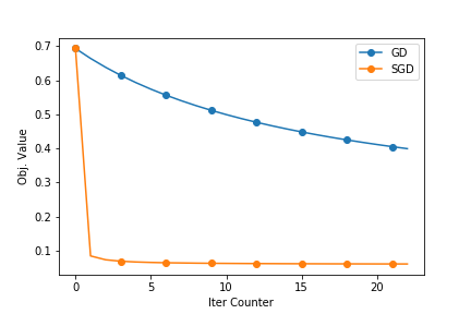
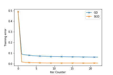
The following plots show how good the SGD is. The dataset used is enron.libsvm. The first plot shows the objective function value and the second ones shows the reduction in training errors as the iterations pass.
The next blogpost will have the Stochastic Gradient Descent (SGD) Implementation. I will try to compare this with SGD. You can find the full source at github